Introduction
Magnetotellurics
At least some books and many scripts about Magnetotellurics are available; Alan Chave & Alan Jones have written a comprehensive book.
Timeseries
We will dive into what we call timeseries - in terms what WE have!
- The data we have is finite. We have a start time and a duration.
\(\Rightarrow\) we always have a cutout of the reality - not the reality itself
\(\Rightarrow\) the data is incomplete \(\Rightarrow\) in terms of the spectral domain: we always have a box function - which limits the resolution of the spectra. - Every sensor has an analogue resolution. A film has a grain, a CCD pixels. A coil as self-noise caused by the electrons moving through the copper. The coil has a self-induction - caused by the currents flowing through the wires, inducing a magnetic field.
- The pre-amplifier is bandwidth limited and has its own noise level. An amplifier can technically not amplify all frequencies. In audio we specialize form 20 Hz to 20 kHz. In MT we have a frequency range from 105 to 10-5 Hz. Transistor based amplifiers have a so called \(\frac{1}{Hz}\) “one over f” noise. Lower frequencies are amplified with higher noise (lucky wise in MT lower frequencies (or longer periods) have higher amplitudes, which lead to a fair compensation).
- The ADC (analogue digital converter) has a quantization noise; especially voltages around the LSB (least significant bit) may be poorly defined (so called bit noise).
- We not only record the signal of interest. We have anthropogene noise - at least the 50 / 60 Hz
Strategy:
- Record long time! As longer you record, as closer you get to the “reality”
- Stacking - more data, more stacks.
Random distributed noise form system amplifiers and sensors will vanish or get smaller.
Temporary noise (short disturbances) will be diminished.
Your recordings are too short! The placement of your station is wrong: you do not have short disturbances, you permanently have disturbances.
MT algorithms are improving. But one relation stays forever true: no input \(\Rightarrow\) no output.
When you acquire data in the field make QC (quality control) a.s.a.p
Remote Referencing improves the data quality.
When you can’t process the data in the field: do not believe that later post-processing is doing much better.
Looking at a crumb cake of data indicates that your data is lost.
Coils
(ref. also Sensors)
The MFS-XX coils are magnetic field sensors which transform a magnetic field variation into a varying output voltage.
All induction coils are following the principle that the output voltage corresponds to the time derivative (or frequency) of the magnetic field $V = $
Therefore \(V \rightarrow 0\) for $ $ for long periods.
This is a) compensated by the fact that lower periods have a greater amplitude, b) that you build a longer coil with more windings and c) design an amplifier which is chopper stabilized in order to reduce the \(\frac{1}{f}\) noise which every amplifier has.
The MFS-06e coil can measure periods down to 4096 s and more (10,000 s). Remote referencing is helpful when calculating the spectra because \(Hx \otimes Hx_r\) reduces the inherent noise.
However: For longer periods coils can’t be used. A fluxgate is needed.
On the upper side at high frequencies eddy currents and self induction degrade the output signal.
A smaller coil with less windings has to be used for frequencies above 1 kHz.
The MFS-07e and SHFT-03e & SHFT-02e are made for AMT and above.
The MFS-07e is good even for 100 s and 1000 s. In resistive areas this corresponds to a depth of 4-10 km. With frequencies up to 50 kHz you can resolve the shallow structure in detail.
Fluxgates
Despite the manufactures data sheets the fluxgates are not suitable for MT above 30 s period.
Fluxgates in technical applications measure active sources which have a much higher field strength than the passive MT field.
For semi airborne measurements an active source is used.
Hence that the sensor output voltage does not drop down at low frequencies. Use auto for gain or manually use 1 or 4 (max).
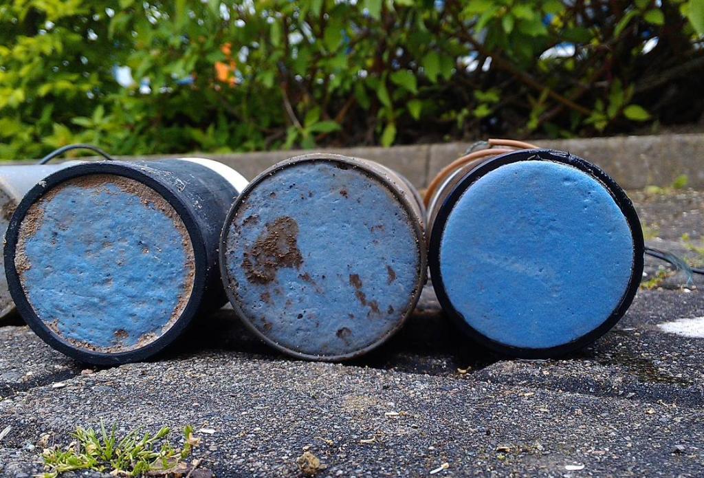
Electrodes
For MT you use non-polarizable electrodes like the EFP-06.
What does non polarizable in simple words? Imagine there is an electric field pointing to North for one hour. If the electrode is chargeable the electrons are now accumulate at the North position.
Now the field suddenly changes to South. In case of a polarizable electrode the “North electrons” first needs to be destroyed, then the electrode is neutral, and after that the electrode sees the South electric field. The electrode does not follow the electric field immediately.
For frequencies above 1 Hz this does not happen. You can use metal sticks for recording.
Always use 5 electrodes of the same type. 4 for the electric field, one for grounding. Therewith you avoid electro chemical voltage between the electrodes.
Use fresh electrodes. Electrodes aging after manufacturing1.
Two years is the given time for Pb/PbCl2 electrodes (EFP-06).
Others like Ag/AgCl electrodes (EFP-07) have a lifetime of > 6 years. However the “half-cell” as well as the ceramic inlet may age.
The noise level increases secretly. You will not notice it in the field immediately! But sooner or later the data below 10 Hz becomes unusable.
Systems
The ADU systems (analoge digital unit). For frequencies above 4 kHz usually 24-bit ADCs are used (and fortunately the dynamic range is small here), and for lower frequencies 32-bit ADCs are used. The greater dynamic range is not driven by the amplitude of the fields but mainly by the drift of the electric field. The drift is caused either by geochemical effects or the electrode itself, and can be 100 times greater than the MT signal. For more details, see 32 or 24 bit ADCs.
Summary
In MT we have a frequency range from 105 to 10-5.
Footnotes
an electro-chemical process is starting after manufacturing; so, like with fresh bread: buy it when you want to eat it.↩︎