Spectral Density

This files contains text and pictures from Siemens[1].

During digital data acquisition, sensors output analog signals which must be digitized for a computer. A computer cannot store continuous analog time waveforms like the sensors produce, so instead it breaks the signal into discrete ‘pieces’ or ‘samples’ to store them.

Data is recorded in the time domain, but often it is desired to perform a Fourier transform to view the data in the frequency domain. There are unique terms used when performing a Fourier transform on this digitized data, which are not always used in the analog case. They are listed in Figure 1 below:

Fig. 8 Time domain and frequency domain terms used in performing a digital Fourier transform[1]

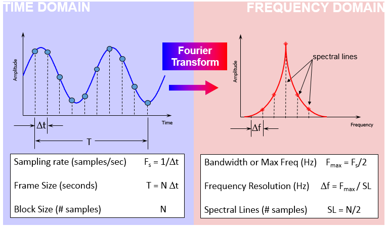
Whether viewing digital data in the time domain or in the frequency domain, understanding the relationship between these different terms affects the quality of the final analysis.

These Digital Signal Processing (DSP) terms and relationships are covered in this article:

1. Time Domain Terms

   1. Sampling Rate (\(f_s\)) – Number of data samples acquired per second

   2. Block Size (\(N, wl, rl\)) – Total number of data samples acquired during one frame, window length (\(wl\)) - Number of samples (+ padding) used for the FFT

   3. Frame Size (\(T\)) – Amount of time data collected to perform a Fourier transform

2. Frequency Domain Terms

   1. Bandwidth (\(bw\)) – Highest frequency that is captured in the Fourier transform, equal to half the sampling rate (analysis bandwidth, we don’t use here) or for DFT \(f_s/N\) (bin width)

   2. Spectral Lines (SL) – After Fourier transform, total number of frequency domain samples (lines)

   3. Frequency Resolution (\(Δf\)) – Spacing between samples in the frequency domain

3. Power Spectra - and Amplitude Spectra Density

Important Note

We use \(wl\) (window length) and \(rl\) (read length). At the beginning both are the same. So both terms are used in the sense \(wl = rl = N\). Later we may do zero Padding . In that section we come to the case \(wl > rl\).

Time Domain Terms

Incoming signals are converted to digital format in the time domain

There are three important settings for time domain digitization: sampling rate, block size, and frame size.

1.1 Sampling Rate (\(f_s\))

Sampling rate (sometimes called sampling frequency or \(f_s\)) is the number of data points acquired per second.

A sampling rate of 1024 samples/second means that 1024 discrete data points are acquired every second. This can be referred to as 1024 Hertz sample frequency.

The sampling rate is important for determining the maximum amplitude and correct waveform of the signal as shown in Fig. 9.

Fig. 9 In the top graph, the 180, 102, 64 Hz sine waves sampled at 1024 samples/second. 102 and 64 Hz have correct amplitude and waveform. In the first plot, 180 Hz, lower sample rates do not yield the correct amplitude nor shape of the sine wave (all sine wave have added 1% noise)

To get close to the correct peak amplitude in the time domain, it is important to sample at least 10 times faster than the highest frequency of interest. For a 102 Hertz sine wave, the minimum sampling rate would be 1024 samples per second. In practice, sampling even higher than 10x helps measure the amplitude correctly in the time domain; in the middle plot the maximum and minimum are not perfectly digitized.

It should be noted that obtaining the correct amplitude in the frequency domain only requires sampling twice the highest frequency of interest. In practice, the anti-aliasing filter in most data acquisition systems makes the requirement 2.5 times the frequency of interest (we use 4 times). The Bandwidth section contains more information about the anti-aliasing filter.

The inverse of sampling frequency (\(f_s\)) is the sampling interval or \(Δt\). It is the amount of time between data samples collected in the time domain

\[\frac{1}{Δt} = f_s\]

The smaller the quantity Δt, the better the chance of measuring the true peak in the time domain.

Note

In the time domain sampling frequency should be 10x higher as the highest frequency of interest in order to get the correct amplitude.

In the frequency domain sample at least 2x higher than the highest frequency of interest; when using standard aliasing filters a factor of 2.5 of higher is needed. In MT we use a factor of 4 (see below)

1.2 Block Size, Window Length (\(N, wl\))

The block size (\(N\)), also called read length (\(wl\)) is the total number of time data points that are captured to perform a Fourier transform. A block size of 1024 means that 1024 data points are acquired.

1.3 Frame Size (\(T\))

The frame size is the total time (\(T\)) to acquire one block of data. The frame size is the block size divided by sample frequency

\[T = \frac{N}{f_s} = \frac{wl}{f_s}\]

Zero Padding does not change the length of the data acquisition - in this case the data was already acquired.

The total time frame size is also equal to the block size times the time resolution.

\[T =N * Δt\]

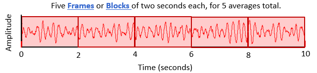
When performing averages on multiple blocks of data, the term total amount of time might be used in different ways (Figure 3) and should not be confused:

• Total Time to Acquire One Block – The frame size (T) is the time to acquire one data block, for example, this could be two seconds

• Total Time to Average – If five blocks of data (two seconds each) are to be averaged, the total time to acquire all five blocks (with no overlap) would be 10 seconds

Fig. 10 Five averages (or stacks) of 2 second frames[1]

Frequency Domain Terms

Incoming signals are converted to digital format in the time domain.

There are three important settings used in the conversion of digital time data to the frequency domain: bandwidth, spectral lines, and frequency resolution.

2.1 Bandwidth (bw)

(there is a term called analytical bandwidth which is different - we do not use it here[2]). The bandwidth is defined as:

\[bw = \frac{f_s}{N} \]

A bandwidth of 1 Hertz means that the sampling frequency is 1024 samples/second, N samples are collected (T = 1s). If you take 2048 samples (T = 2s) at the same sampling frequency of 1024 Hz, the bandwidth is 0.5 Hertz. so theoretically the bandwidth can get very small with large N (or T).
In fact, in reality the ADCs (Analog to Digital Converters) have limitations. At a sample rate of 1024 Hz, the ADC samples a bin within 9.77E-4 seconds. In case this is a CCD sensor and you assume a constant flow of photons, you may guess that you can “divide” the bin further on. Now imagine that the incoming signal is changing within that time frame - you can not “know” what happened within that time frame, like a stroboscope, which appears only in the second half of the bin.
In MT we sample statistical signals. And we later (mostly) stack them. This allows us to increase the bandwidth in case we need it (in order to ged rid of nearby unwanted frequencies). Naturally you also increase the number of stacks when increasing N.

Hence that in many cases the Nyquist frequency ( \(f_s/2\) ) is still affected by the anti aliasing filter of the ADC.

Fig. 11 At 80% of the bandwidth, a anti-aliasing filter starts reducing the amplitude of the incoming signals. The ‘Span’ represents the frequency range without any anti-aliasing filter effects - here shown at 2kHz.[1]

Note

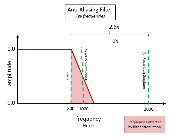
In MT the anti aliasing filters can not be optimized. The input or contact resistance is unpredictable; e.g. for wet soil 100 \(\Omega m\) and for dry terrain up to 10 k\(\Omega m\). Therefore the best practice is to use \(\frac{f_s}{4}\) = 256 Hz at a sample rate of 1024 Hz for interpretation.

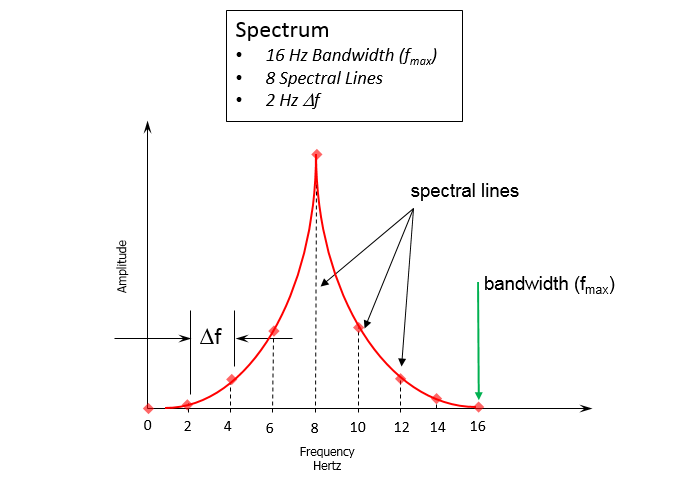
2.2 Spectral Lines (SL)

After performing a Fourier transform, the spectral lines (SL) are the total number of frequency domain data points. This is analogous to N, the number of data points in the time domain. There are two data ‘values’ at each spectral line – an amplitude and a phase value.

Note that while the Fourier Transform results in amplitude and phase, sometimes the frequency spectrum is converted to a power spectral density (PSD) or amplitude spectral density (ASD), which eliminates the phase.

The number of spectral lines is half the block size

\[SL = \frac{N}{2} \]

For a block size of 1024 data points, there are 512 spectral lines and a DC component (0 Hz is not a frequency).

Attention

Some DFTs like the FFTW return a vector / array of 513 for N = 1024. Index[0] is the DC part which can / should be made zero by detrend the window.

2.3 Frequency Resolution

The frequency resolution (Δf) is the spacing between data points in frequency. The frequency resolution equals the bandwidth divided by the spectral lines.

(1)\[ Δf = \frac{f_s}{N} \]

For example, a bandwidth of 16 Hertz with eight spectral lines, has a frequency resolution of 2.0 Hertz.

Fig. 12 Frequency resolution equals bandwidth (bw, Nyquist) divided by spectral lines (SL)[1]

Over all:

(2)\[ \frac{1}{T} = \frac{bw}{SL} = \frac{f_s}{wl} = \frac{f_s}{N} = Δf \]

When spectra needs to be compared ensure that you have the same frequency resolution \(Δf\).

This means that:

• The finer the desired frequency resolution, the longer the acquisition time

• The shorter the acquisition time, or frame size or wl in case the data was already acquired, the coarser the frequency resolution

For higher resolution you need longer recordings:

• 10 Hz frequency resolution is desired, only 0.1 seconds of data is required

• 1 Hertz frequency resolution requires 1 second of data

• 0.1 Hertz frequency resolution requires 10 seconds of data

• 0.01 Hertz frequency resolution requires 100 seconds of data!

Power Spectral Density (PSD)

PSD = ASD². We will handle both together.

Amplitude Spectral Density (ASD)

A Power Spectral Density (PSD) is the measure of signal’s power content versus frequency. A PSD is typically used to characterize broadband random signals. The amplitude of the PSD is normalized by the spectral resolution employed to digitize the signal.

Important

The DEFAULT scaling of 1D FFT of REAL DATA (not complex input numbers) of the FFTW is scaled (multiplied) with:

(3)\[\frac{1}{(wl \big/ 2)} = \frac{1}{(T \big/ 2)}\]

due to conjugate symmetry 1/2 of the FFT result is not used see FFT Units. An alternative scaling is RMS, which is \(\sqrt{2}\) for a sine wave.

For magnetic and electric field data, a PSD and ASD have amplitude units of

(4)\[\begin{split} \begin{aligned} \frac{nT^2}{Hz} && \text{and} && \frac{nT}{\sqrt Hz} \\ \left(\frac{mV}{km}\right)^2 /Hz && \text{and} && \frac{mV}{km \sqrt Hz} \end{aligned} \end{split}\]

The ASD can be related to terms of Standard Deviation of the signal level.

Important

The DEFAULT scaling of ASD is

\[\sqrt{\frac{1}{T/2 \cdot f_s²}} = \sqrt{\frac{1}{T \cdot bw \cdot f_s}} = \sqrt{\frac{1}{wl / 2 \cdot f_s}} \]

While this unit may not seem intuitive at first, it helps ensure that random data can be overlaid and compared independently of the spectral resolution used to measure the data.

Hint

In MT we measure NOISE data - not sine waves. 99.99% of all FFT / DFT tutorials are about (infinite) sine waves like we have with 50 Hz or 60 Hz waves. This is exactly not what we analyze. Schumann resonances may be the exception.

To understand a Amplitude Spectral Density (ASD), it is helpful to understand some limitations of an autopower function when analyzing data with differing spectral resolutions:

Fig. 13 0.1% noise with the sine waves, rl 1024 - not ASD scaled

Fig. 14 0.1% noise with the sine waves, rl 1024 - ASD scaled

Fig. 15 0.1% noise with the sine waves, rl 4096 - not ASD scaled

Fig. 16 0.1% noise with the sine waves, rl 4096 - ASD scaled

It is evident that a) either the amplitude of the sine wave is constant OR b) the noise level appears to be constant.

In the figures above the frequency resolution \(\Delta f\) changes from 1 Hz to 0.25 Hz.

Fig. 17 Different \(\Delta f\) bin sizes[1]

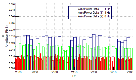
For a sine wave with a single frequency this does not matter as shown below:

Fig. 18 Different \(\Delta f\) bin sizes for a single frequency[1]

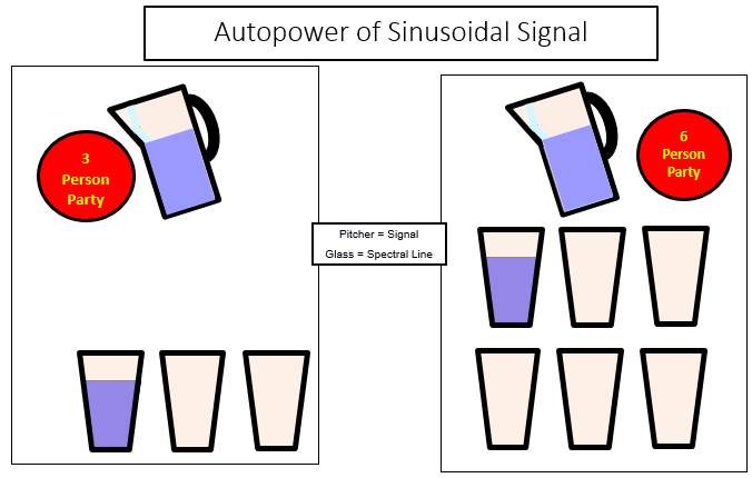
As long as the sampling rate is 4 x higher as the target frequency and the spectral resolution \(\Delta f\) is 2 x then the neighboring sine waves are, there will be only one bin for one frequency. In the figure above in spectral resolution increased by 2 ( \(\Delta f \Rightarrow \Delta f/2 \) ). … hence the other direction ( \(\Delta f/2 \Rightarrow \Delta f \) ) is limited!

For noise signals like in MT this is NOT true. In case of all frequencies (“white noise”) each \(\Delta f\) picks up a smaller and smaller segment of data.

Fig. 19 Different \(\Delta f\) bin sizes for a noise signal[1]

Where as in sinusoidal Figure only one glass gets filled up with exactly one frequency, here several frequencies share either three or six glasses and - nicely displayed - they have not the same filling level anymore[3]

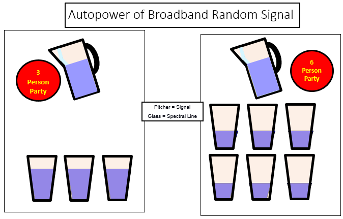
The amplitude spectral density (ASD) solves that problem by normalizing the bins by \( \frac{1}{\sqrt Hz} \) (and PSD \( \frac{1}{Hz} \) )

Where now the noise (or random) signal appears independent from \(T\) or \(wl\) and therewith the duration of observation and respectively \(\Delta f\) - the “sine wave has a problem”: the former rule “one bin one frequency” stays true - but - the bin is now scaled by \(\frac{1}{\sqrt Hz}\) dependent on the spectral resolution \(\Delta f\).

For MT this isn’t a problem because we do not have periodic data (except maybe Schumann resonances). The typical 16 2/3, 50/60 Hz and others are excluded from processing.

MT is NOT White Noise

Not all frequencies are generated by the Sun-Earth system. Especially to mention the so called AMT gap between 1 - 3 kHz. And the timeseries are limited.

Zero Padding

Zero Padding

FFT Units

Lets look a a signal with the unit V, the complex spectra:

\[ Cspectra(f) = \int_{t_1}^{t_2} sample(t) e^{ 2\pi ift} \,dt \]

the samples(f) are integrated over time and the unit is now

\[ [V s] = [V/Hz] \]

for a two sided complex spectrum.

The peak value of the spectrum now depends on the time measured / used / integrated; as above (3) we can scale by \(T/2\) and get a simple one-sided scaled amplitude spectrum:

\[ [V] \]

For a one-sided real spectral power density we do

\[ PSD(f) = 2 \bigl| Cspectra(f) \bigr|^2 \big/ (t_2 - t_1) \]

\[ V s \Rightarrow \frac {V^2 \cdot s^2}{T} = V^2 s = \big[ V^2 \big/ Hz \big]\]

or taking the square root for getting the spectral amplitude density (ASD)

\[ \big[ V / \sqrt{Hz} \big] \]

for the sake of completeness

\[ T := t_2 - t_1 ; \Rightarrow 2 \cdot (\dots) \big/ T = \frac {1}{T/2}\]

---

[1] (1,2,3,4,5,6,7,8)

The Siemens Tutorial is an excellent source. It has been modified slightly for the needs of MT

[2]

Analytical bandwidth is \(f_s/2\) . That is the maximum frequency that can be analyzed without aliasing, Nyquist frequency. We don’t use that for the DFT - there we use \(f_s/N\) as bin width and bandwidth.

[3]

For a mathematical FFT the integral can be infinite with a endless frequency resolution … but who as time? We always “living in a box”